Lower Bound OP

A problem we have encountered in Analyze is that we are frequently surfacing OP rates with a very low % of Medicare. To identify outlier rates, we use a medicare bound (5%) or rely on validated rates’ IQR-based benchmarks.

Mostly Surgical Codes

Code

df = pd.read_sql(f"""
SELECT
   is_surg_code,
   count(*) as n
FROM tq_dev.internal_dev_csong_cld_v2_2_1.prod_combined_abridged df
WHERE canonical_rate_percent_of_cbsa_avg_medicare < 0.6
AND bill_type = 'Outpatient'
GROUP BY 1
""", con=trino_conn)
df['percent'] = df['n'] / df['n'].sum()
df

is_surg_code	n	percent
	4894052	0.133937
True	31645957	0.866063

Percent of ROIDs that are outliers

Code

df = pd.read_sql(f"""
SELECT 
    is_surg_code, 
    count(*) as n,
    SUM(
        CASE
            WHEN canonical_rate_percent_of_cbsa_avg_medicare < 0.6 THEN 1
            ELSE 0
        END
    ) as n_outlier
FROM tq_dev.internal_dev_csong_cld_v2_2_1.prod_combined_abridged df
WHERE bill_type = 'Outpatient'
GROUP BY 1
""", con=trino_conn)
df['perc'] = df['n_outlier'] / df['n']
print(df.to_markdown(index=False))

is_surg_code	n	n_outlier	perc
True	211497323	31645957	0.149628
	749629244	4894052	0.00652863

---

Codes where p25 of Validated Rates AND Allowed Amounts Benchmarks are below Medicare

Code

# %%
df = pd.read_sql(f"""
WITH
allowed_amounts AS (
    SELECT 
        state,
        tq_payer_id,
        billing_code,
        AVG(percentile_25th) AS percentile_25th,
        AVG(median_allowed_amount) AS median_allowed_amount
    FROM tq_production.claims_benchmarks.claims_benchmarks_allowable_state_payer
    WHERE 
        payer_channel = 'Commercial'
        AND allowed_amount_type = 'claim'
        AND billing_code_ranking = 'primary'
        AND npi_source = 'hco'
        AND claim_type_code = 'institutional'
        AND setting = 'Outpatient'
        AND billing_code_type = 'HCPCS'
        AND run_date = DATE '2025-10-23'
        AND service_year >= 2024
    GROUP BY 1, 2, 3
)
SELECT 
    df.billing_code,
    APPROX_PERCENTILE(aa.percentile_25th, 0.5) as p25_allowed_amount,
    APPROX_PERCENTILE(aa.median_allowed_amount, 0.5) as median_allowed_amount,
    APPROX_PERCENTILE(canonical_rate, 0.25) as p25_canonical_rate,
    APPROX_PERCENTILE(canonical_rate, 0.5) as p50_canonical_rate,
    APPROX_PERCENTILE(cbsa_avg_medicare_rate, 0.5) as median_cbsa_avg_medicare_rate
FROM tq_dev.internal_dev_csong_cld_v2_2_1.prod_combined_abridged df
JOIN allowed_amounts aa
    ON df.state = aa.state
    AND df.payer_id = aa.tq_payer_id
    AND df.billing_code = aa.billing_code
WHERE
    canonical_rate_score = 5
    AND bill_type = 'Outpatient'
    AND provider_type = 'Hospital'
    AND is_surg_code = True
GROUP BY 1
""", con=trino_conn)

# %%
df_sample = df.loc[
    (df['p25_canonical_rate'] < df['median_cbsa_avg_medicare_rate']) &
    (df['p25_allowed_amount'] < df['median_cbsa_avg_medicare_rate'])
].copy()
df_sample['diff_percent'] = (
    (df_sample['median_cbsa_avg_medicare_rate'] -
     df_sample['p25_canonical_rate']) /
    df_sample['p25_canonical_rate'] * 100
)
df_sample = df_sample.head(40)

# Calculate percentages relative to medicare rate
df_sample['p25_canonical_pct'] = (
    df_sample['p25_canonical_rate'] /
    df_sample['median_cbsa_avg_medicare_rate'] * 100
)
df_sample['p25_allowed_pct'] = (
    df_sample['p25_allowed_amount'] /
    df_sample['median_cbsa_avg_medicare_rate'] * 100
)
df_sample['medicare_pct'] = 100.0

# df_sample.to_excel('samples.xlsx', index=False)

# %%
# plot
# Reshape data for seaborn
df_plot = df_sample.melt(
    id_vars=['billing_code'],
    value_vars=['p25_allowed_pct', 'p25_canonical_pct'],
    var_name='metric',
    value_name='percentage'
)

# Create more readable labels
label_map = {
    'p25_allowed_pct': 'P25 Allowed Amount',
    'p25_canonical_pct': 'P25 Canonical Rate',
    'medicare_pct': 'Medicare Rate (baseline)'
}
df_plot['metric'] = df_plot['metric'].map(label_map)

fig, ax = plt.subplots(figsize=(12, 16))

sns.barplot(
    data=df_plot,
    y='billing_code',
    x='percentage',
    hue='metric',
    ax=ax,
    palette='Set2'
)

ax.set_ylabel('Billing Code', fontsize=12)
ax.set_xlabel('Percentage of Medicare Rate (%)', fontsize=12)
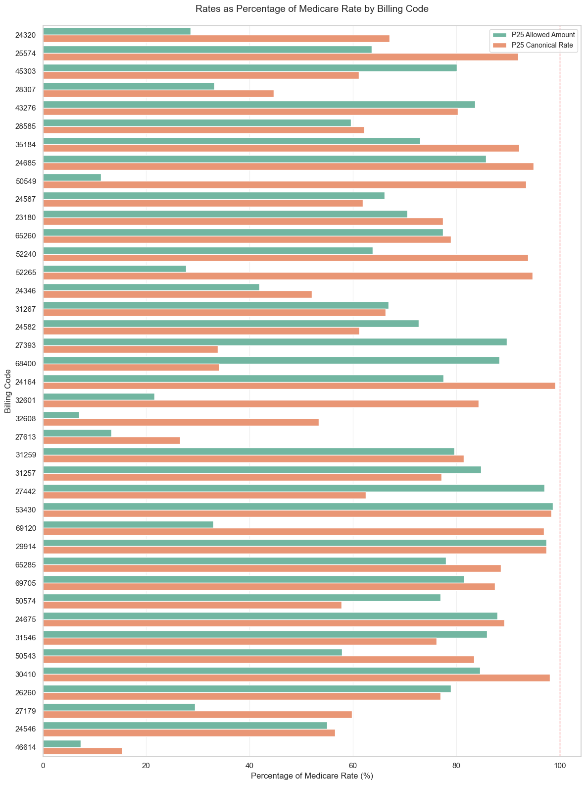
ax.set_title(
    'Rates as Percentage of Medicare Rate by Billing Code',
    fontsize=14,
    pad=20
)
ax.legend(title='', fontsize=10)
ax.grid(axis='x', alpha=0.3)
ax.axvline(x=100, color='red', linestyle='--', linewidth=1, alpha=0.5)

plt.tight_layout()
plt.show()

Deep Dive into Couple Codes

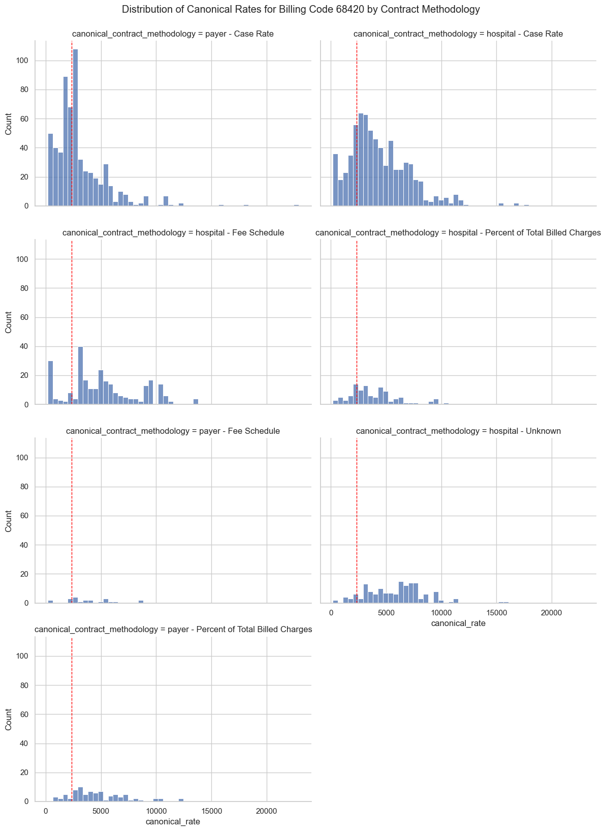
68420

Code

# %%
check = pd.read_sql(f"""
SELECT hcpcs, approx_percentile(rate, 0.5)
FROM tq_production.reference_internal.opps_reference_pricing
WHERE apc = '5503'
AND is_latest_start_effective_date = True
GROUP BY 1
""", con=trino_conn)

# %%
df = pd.read_sql(f"""
SELECT 
    billing_code,
    payer_id,
    provider_id,
    canonical_rate, 
    canonical_rate_type, 
    canonical_rate_source || ' - ' || canonical_contract_methodology as canonical_contract_methodology
FROM tq_dev.internal_dev_csong_cld_v2_2_1.prod_combined_abridged
WHERE billing_code IN ('{"', '".join(check['hcpcs'].tolist())}')
AND bill_type = 'Outpatient'
AND is_surg_code = True
AND provider_type = 'Hospital'
AND canonical_rate_score = 5
""", con=trino_conn)

# %%
mpfs_rates = pd.read_sql(f"""
SELECT hcpcs as billing_code, approx_percentile(facility_rate, 0.5) as mpfs_rate
FROM tq_production.reference_internal.physician_reference_pricing
WHERE hcpcs IN ('{"', '".join(check['hcpcs'].tolist())}')
AND is_latest_start_effective_date = True
GROUP BY 1
""", con=trino_conn)

# %%
df_merged = df.merge(mpfs_rates, on='billing_code', how='left')

# %%
import seaborn as sns
import matplotlib.pyplot as plt
df_code = df_merged[df_merged['billing_code'] == '68420'].copy()
sns.set_theme(style='whitegrid')
g = sns.displot(
    data=df_code,
    x='canonical_rate',
    col='canonical_contract_methodology',
    col_wrap=2,
    bins=50,
    height=4,
    aspect=1.5
)
g.map(plt.axvline, x=2332.96, color='red', linestyle='--', linewidth=1)
g.fig.suptitle('Distribution of Canonical Rates for Billing Code 68420 by Contract Methodology', y=1.02)
plt.show()

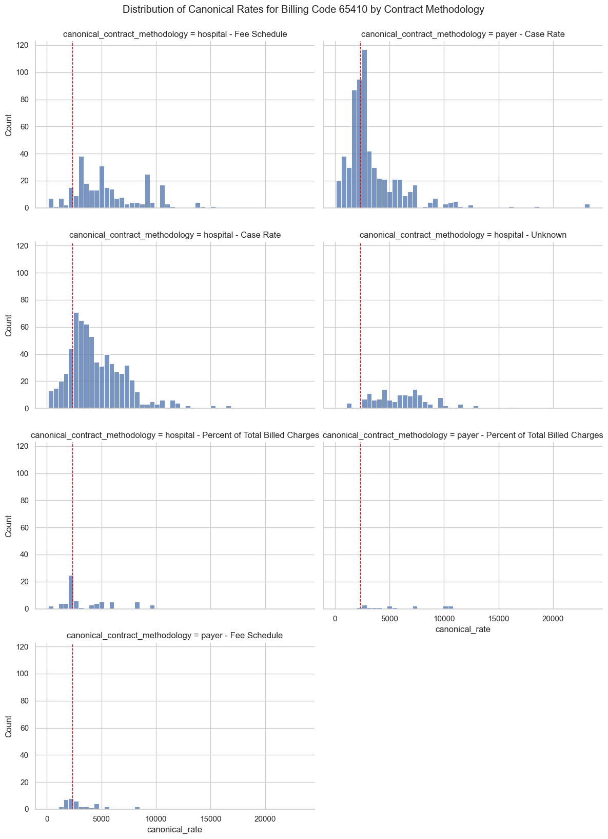
65410

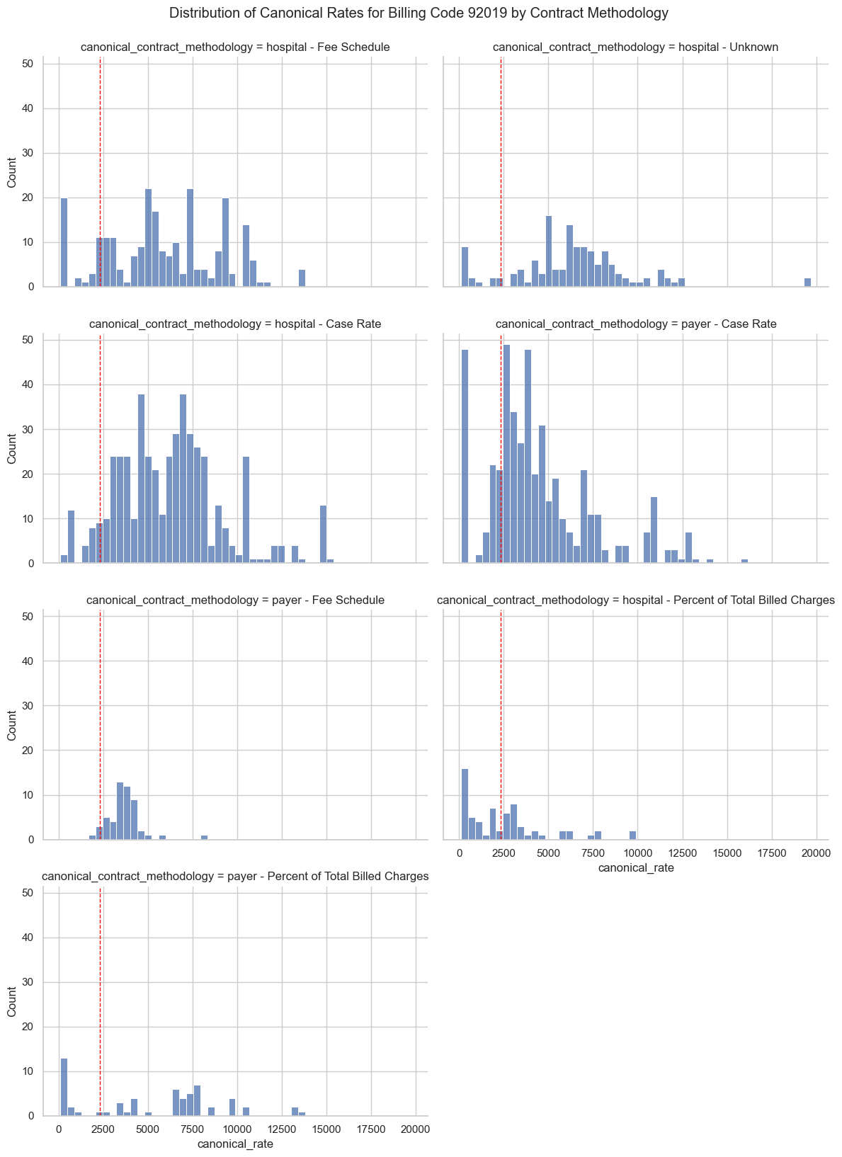
92019

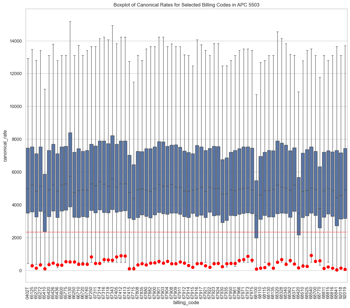
Boxplots for APC 5503