Accuracy Scores v2

Goal:

We explain how validated canonical rates can be used to improve accuracy scoring.

Background:

note

validated = payer and hospital reported similar rates (i.e. < 20% difference)

Given a rate object, there are many potential representations of a rate. As an example, hospital may have posted rates as a percentage, dollar, estimated allowed amount, or multiple rates with different contract methodologies. Payers can similarly post multiple rates.

In this v2 of accuracy scoring, we focus on breaking ties where both hospital and payer have posted rates that are within reasonable medicare benchmarks, but NOT validated (they are more than 20% apart). Until now, we had broken this tie by deferring to data source, e.g. select the hospital rate.

Methodology

Scope

This is v2 and there will be v3, v4 and so on.

For this version:

1. We're only trying to break best "hospital" and best "payer" ties. We're not yet going to use this to pick a best rate when there are multiple rates WITHIN a payer, that are all passing benchmarks.
2. We're only using normal-ish looking distributions. Inferences are harder when non-normal + inferences are less reliable if we assume normal when they are clearly not normal. We want to make sure distributions are not extremely skewed and that they are not multimodal.
3. We're going to generate validated canonical rate distributions NATIONALLY (or bucket hospitals into "high", "medium" and "low" cost). We lose sample sizes as we make the cohort more granular.

Steps

1. Pull all validated rates
2. Log transform the rates to reduce skew
3. For each billing code, calculate skewness and kurtosis.
   • Skewness measures the symmetry of a distribution
   • Kurtosis measures how heavy the tails of a distribution are (it roughly tells us how flat it is).
4. Exclude distributions that are extremely skewed or have kurtosis < -0.75
5. Estimate the median and variance of the distributions.
6. In the Clear Rates pipeline:
   • add a step in accuracy to approximate the likelihoods of observing the rate given the validated distribution (for more details see Likelihood Estimation section at bottom of this page)
   • in case of payer/hospital ties, select the rate that is closer to the median

Summary

We exclude ~600 billing codes due to low kurtosis:

low_kurtosis
False    6963
True      590

We exclude ~7 billing codes due to extreme skew:

high_skew
False    7546
True        7

Examples

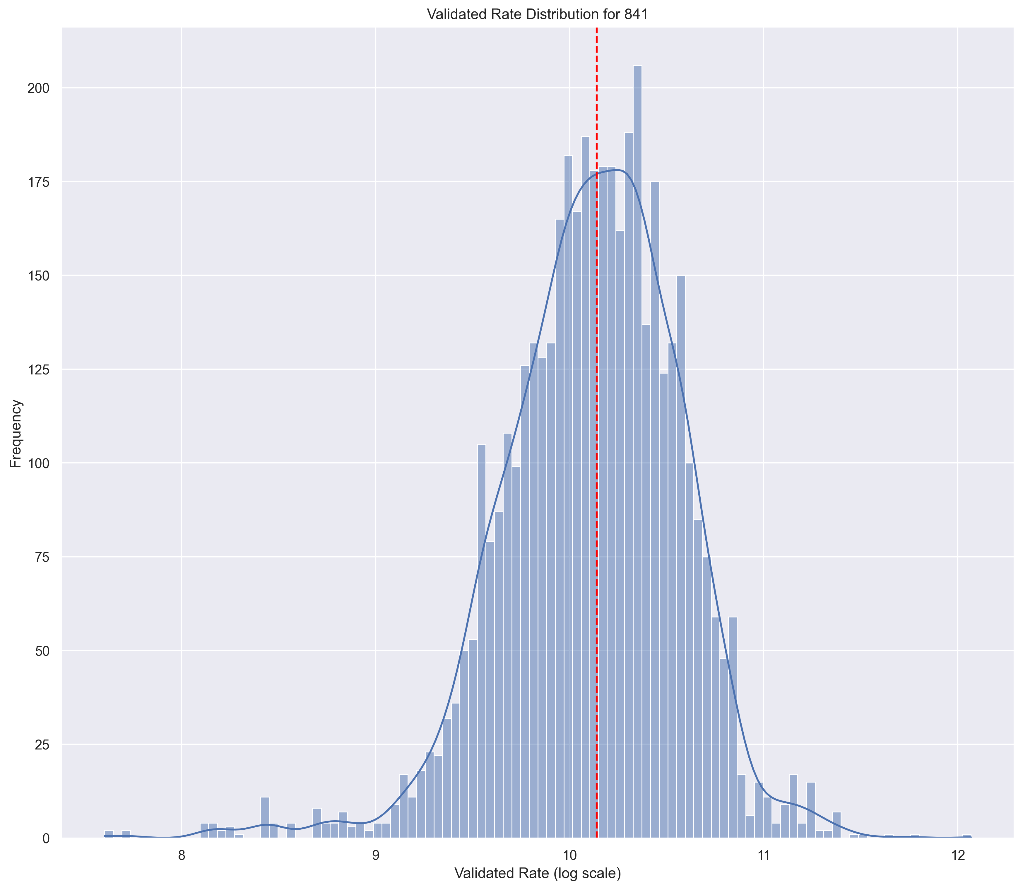
Good Distribution

skewness = -0.080498 
kurtosis = -0.258124

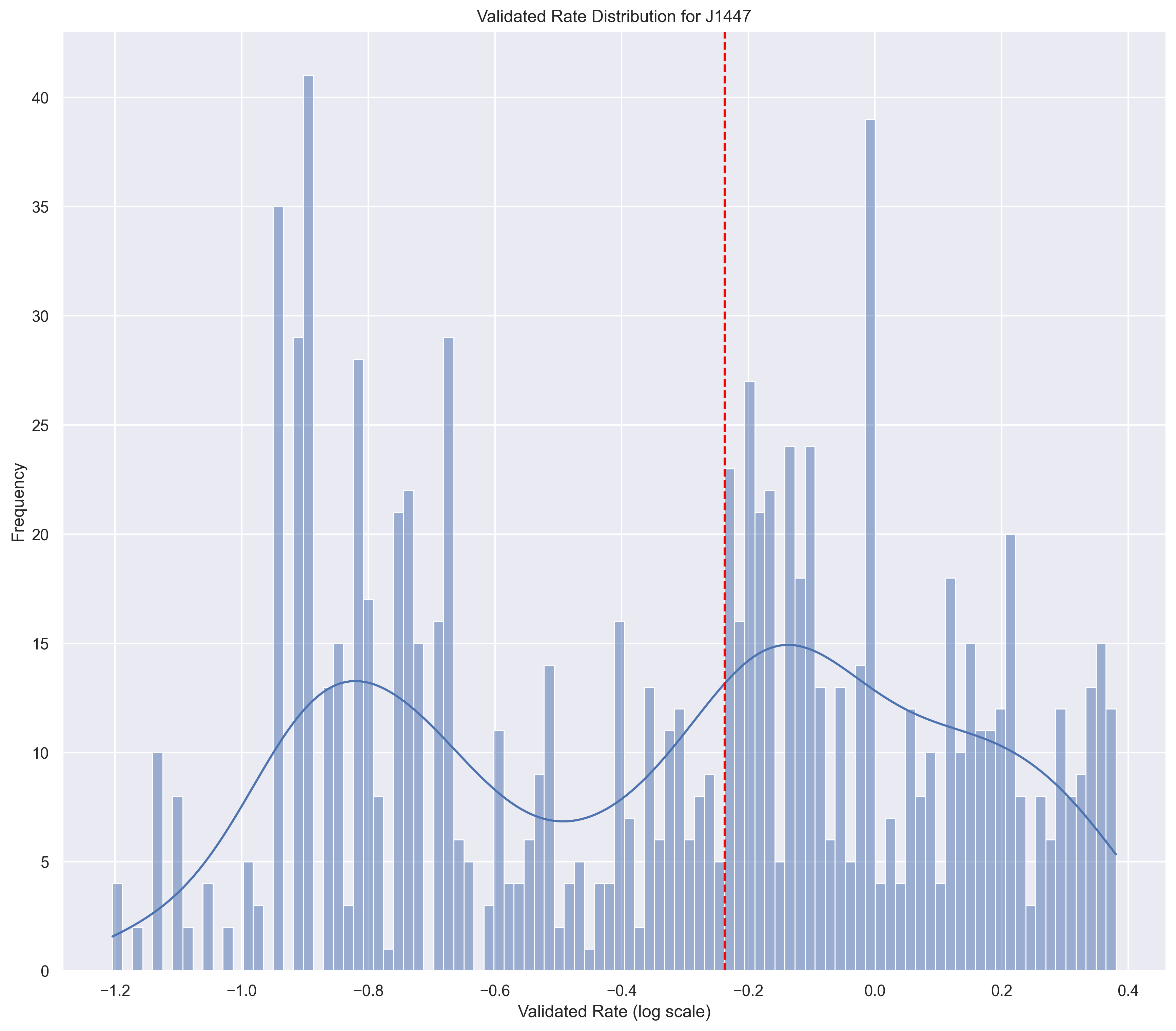
Bad Distribution

skewness = 0.395
kurtosis = -0.973

note

These "bad" distributions may be informative. If the distribution is bi-modal, what's going on? Is that real? Is it due to our omission of contract methodology-based pricing? Is it due to dosage standardization?

Likelihood Estimation

Goal

The goal is to offer a statistic that can interpreted in the following way:

The $1200 rate has a likelihood of 0.36. The probability of observing this value from a random draw is 36%.

We want to estimate the likelihood of observing a rate $x$ given a normal distribution with parameters $\mu$ and $\sigma$.

To approximate, we'll use:

$\mathrm{CDF}(b) - \mathrm{CDF}(a)$

where b = rate + $\epsilon$ and a = rate - $\epsilon$.

This is just the integral of the probability distribution function over a range near the rate.

In SQL, we can use this MACRO:

{% macro normal_cdf_of_range(col) %}
   {% set epsilon = '0.05 * ob.median' %}
   {% set lower_bound = 'LEAST(ln(r.' ~ col ~ ') - ' ~ epsilon ~ ', ln(r.' ~ col ~ ') + ' ~ epsilon ~ ')' %}
   {% set upper_bound = 'GREATEST(ln(r.' ~ col ~ ') - ' ~ epsilon ~ ', ln(r.' ~ col ~ ') + ' ~ epsilon ~ ')' %}
   ABS(
      normal_cdf(ob.median, ob.stddev, {{ lower_bound }}) 
      - 
      normal_cdf(ob.median, ob.stddev, {{ upper_bound }})
   )
{% endmacro %}